Modes of SimBA

SimBA assists the user in analyzing and optimising electrified bus fleets and schedules. Besides a simple simulation run, several different modes support the user in finding optimal solutions for their eBus-System. Supported modes are

• simple simulation

• negative depot to opportunity charger

• negative opportunity to depot charger

• service optimization

• station optimization

• report

• remove negative rotations

Chained Modes

While the default mode of SimBA is the simple simulation together with a report, modes can be chained together differently to achieve the desired results. The chain of modes is defined in the config file (default: simba.cfg) under the keyword mode:

mode = ["sim", "report"]

This results in a simple simulation with a following report. To run a simulation SimBA creates a schedule which contains all information about how the bus system is supposed to run. Some modes are allowed to mutate the schedule in some way, which makes chaining of modes especially useful. Their output describes the simulation outcome of this mutated schedule. An extended simple use case would be:

mode = ["sim", "report" ,"neg_depb_to_oppb", "remove_negative", "report]

Where the scenario is run as is, a report is generated, the schedule is changed and simulated again and a second report is generated. Descriptions for the modes can be found below.

Simple Simulation

mode = ["sim"]

The simple simulation case is the default mode. Its usage is explained in Getting Started. Every chain of modes starts with a simple simulation, even if it is not explicitly listed in the modes. The simulation takes the scenario as is. No parameters will be adjusted, optimized or changed in any way. The charging type for each vehicle is read from the rotation information from the trips.csv if this data is included. If the data is not included preferred_charging_type from the config file is used, as long as the provided vehicles data provides the preferred_charging_type for the specified vehicle type.

Negative Depot to Opportunity Charger

This mode is the first kind of optimization provided by SimBA and is called by:

mode = ["neg_depb_to_oppb"]

It takes the results of the previous simulation, and changes the charging type of all rotations which had a negative SoC to opportunity chargers.

Note

Charging types are only switched by SimBA if the corresponding vehicle type as opportunity charging bus exists in the provided vehicles_data.json.

Negative Opportunity to Depot Charger

This mode is analogous to neg_depb_to_oppb. This mode is the second kind of optimization provided by SimBA and is called by

mode = ["neg_oppb_to_depb"]

It takes the results of the previous simulation, and changes the charging type of all rotations which had a negative SoC to depot charging.

Note

Charging types are only switched by SimBA if the corresponding vehicle type as depot charging bus exists in the provided vehicles_data.json.

Service Optimization

It can happen that several buses influence each other while simultaneously charging at the same charging station, e.g. due to limited grid power or limited number of charging stations, which can lead to negative SoCs due to hindered charging. In this case, this mode finds the largest set of rotations that results in no negative SoC. This is done by first taking all rotations that do become negative and finding their dependent rotations, i.e., ones that can have an influence by sharing a station earlier with the negative rotation. Next, all rotations are filtered out that stay negative when running with just their dependent rotations. Now, only rotations are left that are non-negative when viewed alone, but might become negative when run together. To find the largest subset of non-negative rotations, all possible set combinations are generated and tried out. When a union of two rotation-sets is non-negative, it is taken as the basis for new possible combinations. The previous two rotation-sets will not be tried on their own from now on. In the end, the largest number of rotations that produce a non-negative result when taken together is returned as the optimized scenario.

Station Optimization

Greedy Optimization

This mode optimizes a scenario by electrifying as few opportunity stations as possible using a greedy approach. Two basic approaches to use the optimization module are setting the mode in the SimBA configuration file to

mode = ["sim", "station_optimization", "report"]

or

mode = ["sim","neg_depb_to_oppb", "station_optimization", "report"]

While the first call optimizes the scenario straight away trying to electrify all opportunity chargers, the second call, changes depot chargers to opportunity chargers, if they were not able to finish their rotations in the first simulation run. This way the second approach can lead to a higher degree of electrification for the system. The network with no opportunity charging station is first analyzed to find rotations which fail at the current stage and to estimate the potential of electrifying each station by its own. Step-by-step new opportunity stations are electrified until full electrification is reached. The optimization assumes that at every newly electrified station unlimited charging points exist, i.e. the number of simultaneously charging buses is not limited. In between each electrification a simulation is run and the network is analyzed again. The first run called the base optimization leads to a scenario which often times is better than extensively optimizing the scenario by hand. Since a greedy approach can not guarantee a global optimum a second extensive optimization can be chained to this base optimization. This deep optimization can make use of a step-by-step decision tree expansion which evaluates new combinations of electrified stations starting with the most promising combinations OR use a brute force approach trying to reduce the amount of electrified stations by one in comparison to the base optimization. The step-by-step process of the optimization follows Fig. 3

Fig. 3 Steps of the optimization loop until full electrification is reached.

After a single simulation is run the rotations are analyzed. Any time a vehicle goes below an SoC of zero (or a self defined value) a low SoC event is triggered. This event saves information about when the SoC reached its minimal value and the history before that up to a point of an upper SoC threshold, with the default value being 1. Stations inside of this time span are potentially able to mitigate the low SoC and are stored with other information about the event. Fig. 4 shows a possible SoC history with a low SoC event.

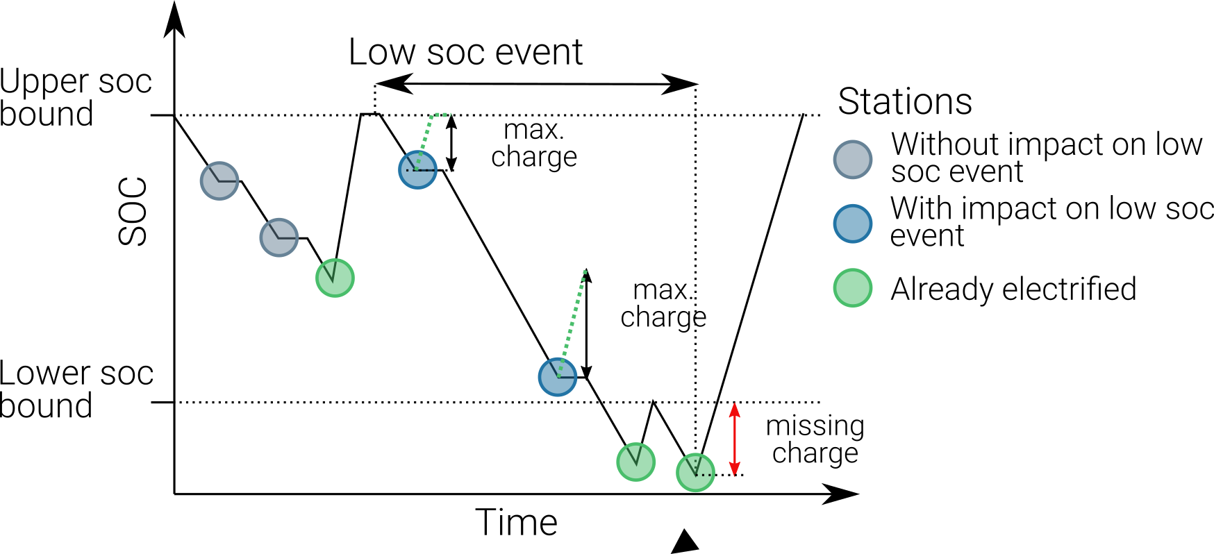
Fig. 4 Low SoC event and classification of stations.

The next step groups low SoC events based on the stations which were found earlier. Events which share at least one station could possibly interact with each other, e.g. vehicles could share a charging station. Therefore, groups are build which do not share any stations in between groups. This speeds up the optimization process since for every electrification and simulation only rotations are calculated which could be impacted by the change.

Since greedy approaches execute the step which seems most promising in the current situation an evaluation function is needed. One possible approach could be to simulate each scenario, meaning simulating every case in which one of all possible stations is electrified and continuing with the best case. The optimizer does not use this approach. Instead, an approximation function is used to evaluate the potential of electrifying a station. This approximation function analyzes the duration at each stop, the possible charging time, the SoC and resulting possible charging power (in general batteries with high SoCs are charged at a lower rate) as well as the upper SoC threshold and minimal SoC of the event. While this methodology is not accurate in all cases, e.g. a station could exist multiple times inside a low SoC event, therefore charging the first time at this station would alter the SoC and charging power the vehicle has the second time it reaches the station, it seems well suited as heuristic for choosing the most promising station. The objective function of choosing what the best station is, is the mitigation of missing charge, i.e. what is the minimal amount of energy that needs to be inserted into the battery, so that no SoC is below 0.

After the evaluation selected a station to be electrified the scenario input data is altered so that vehicles at this station are charged without limitation of charging points. This is followed up by a detailed simulation which can make use of a highly accurate solver for charging events called SpiceEV or a less accurate but faster solver. Now the resulting system has less missing charge and the potentials of stations might be decreased. Also, a single group might have been split up into several smaller groups which can be analyzed even quicker. Therefore, the loop repeats up until the point the missing charge in the system is zero or in other words the system is fully electrified.

At the current stage the scenario to be optimized needs depot charging stations at the start and end of each rotation. The scenario should not contain any opportunity charging stations. If for a given scenario opportunity charging stations are predefined, i.e. the scenario should contain a specific electrification and is set in the electrified_station.json the solver type spice_ev should be used in the optimizer.cfg. If the quick solver is supposed to be used the station can be listed in inclusion_stations while the electrified_stations.json should only contain depot stations. Stations can be also excluded from optimization by adding their name to exclusion_stations.

Deep Optimization

The greedy algorithm in the base optimization can not guarantee that the solution is the global optimum. This is why the use of the deep mode is recommended for systems with high requirements. After the first run, instead of electrifying the station with the highest potential the second-best station is electrified. This is similar to a decision tree, where every node is a set of electrified stations, with the first node being zero stations electrified and the last node being all stations electrified. The nodes in between correlate with every possible state of electrification. Each branch therefore represents an additional electrification of a single station. The algorithm continues electrifying the best station, as long as this node has not been evaluated yet. This way gradually all possible nodes are checked. The search stops whenever the number of stations surpasses the number of the current optimal solution. If several options with the same optimal number of stations arise, they can be found in the log file of the optimizer, but only one file with optimized stations is produced.

Pruning is used to stop evaluation of branches, whenever foresight predicts that no better solution will be reached. This is done through the simple heuristic of checking the sum of potentials of the n remaining stations with the highest potentials, with n being the number until the number of stations of the current optimal solution is reached.

Example:

The base optimization found a set of 5 stations to fully electrify the scenario. These stations are A, B, C, D and E which were chosen in the same order. The whole scenario consists of the whole alphabet of stations. The deep optimization starts with evaluating a scenario without any electrified opportunity stations. Depot stations are electrified. The first evaluation gives a sorted list of potentials by

Station	Potential
A	85
X	75
B	30
E	25
…	…

In the base optimization Station A was chosen since it showed the highest potential. The deep optimization ignores this node since it has been evaluated already and chooses station X instead. After a detailed simulation with X electrified, the remaining stations are evaluated again.

Station	Potential
B	28
E	25
C	20
G	18
…	…

For every vehicle the amount of missing energy is calculated and summed up. In this example case the missing energy is 85. Since 4 stations are remaining until the current optimum of 5 stations is reached, the 4 stations with the highest potential are evaluated in this case

\[Pot = Pot_B + Pot_E + Pot_C + Pot_G = 28 + 25 + 20 +18 = 91\]

In this case the potential is high enough to continue the exploration of this branch. If the potential had been below 85 the branch would have been pruned, meaning it would not be explored any further and labeled as not promising. It is not promising since it will not lead to a better solution than the current one. This is the case since on one hand the evaluation by approximation tends to overestimate the potential while the missing energy is accurately calculated and on the other hand electrification of stations can reduce the potential of other stations, for example if 2 stations charge the same rotation, electrifying one station might fully electrify the rotation meaning the potential of the other station drops to zero. This concept can reduce the amount of nodes which have to be checked.

Other Optimization Functionality

Mandatory stations can be attained to increase the speed of the optimization process. Mandatory stations are defined by being stations which are needed for a fully electrified system. To check if a station Y is mandatory the network with every station electrified except Y is simulated. If the system has vehicle SoCs which drop below the minimal SoC (default value is 0) in this scenario, the station is mandatory. In the later exploration of the best combinations of stations this station will be included in every case.

Impossible rotations are rotations which given the settings are not possible to be run as opportunity chargers, given the vehicle properties, even when every station is electrified. Before starting an optimization it is recommended to remove these rotations from the optimization, since the optimizer will not reach the goal of full electrification.

Quick solver Instead of using the regular SpiceEV solver for optimization the user can also choose the quick solver. This approximates the SoC history of a vehicle by straight manipulation of the SoC data and numeric approximations of the charged energy. Therefore, small differences between solving a scenario with SpiceEV and the quick solver exist. For the quick solver to work, some assumptions have to be met as well

• Depots charge the vehicles to 100% SoC

• Station electrification leads to unlimited charging points

• Base scenario has no electrified opportunity stations

• No grid connection power restrictions

At the end of each optimization the optimized scenario will run using SpiceEV. This guarantees that the proposed solution works. If this is not the case, using SpicEV as solver is recommended

Continuing optimizations can be useful in cases where simulation of the base case is slow or considerable effort was put into optimization before. The user might want to continue the optimization from the state where they left off. To speed up multiple optimizations or split up a big optimization in multiple smaller calculations two features are in early development. Experienced users can use these features on their own accord with a few minor implementation steps. To skip a potentially long simulation, with the simulation of the scenario being the first step of every SimBA run, the optimizer.config allows for using pickle files for the three major objects args, schedule and scenario. After pickling the resulting objects, the optimizer can be prompted to use them instead of using whatever other input is fed into the optimizer. This is done by giving the paths to the pickle files in the optimizer.cfg.

args = data/args.pickle
schedule = data/schedule.pickle
scenario = data/scenario.pickle

If they are provided they are used automatically. All three pickle files need to be set.

If a deep optimization takes to long to run it in one go, it is possible to save the state of the decision tree as pickle file as well. Reloading of the state is possible and will lead to a continuation of the previous optimization. This feature is still in development and needs further testing. To make use of this feature the parameters in the optimizer.cfg have to be set.

decision_tree_path = data/last_optimization.pickle
save_decision_tree = True

Optimizer Configuration

The functionality of the optimizer is controlled through the optimizer.cfg specified in the simba.cfg used for calling SimBA.

Table 1 Optimizer.cfg parameters

Parameter	Default value	Expected values	Description
debug_level	1	1 to 99	Level of debugging information that is printed to the .log file. debug_level = 1 prints everything
console_level	99	1 to 99	“Level of debugging information that is printed in the console. console_level = 99 only prints critical information.”
exclusion_rots	[]	[“rotation_id1”, “rotation_id2” ..]	Rotations which shall not be optimized
exclusion_stations	[]	[“station_id1”, “station_id2” ..]	Stations which shall not be electrified
inclusion_stations	[]	[“station_id1”, “station_id2” ..]	Station which shall be electrified. Note: If using inclusion stations, rebasing is recommended
standard_opp_station	{“type”: “opps”, “n_charging_stations”: 200, “distance_transformer”: 50}	dict()	Description of the charging station using the syntax of electrified_stations.json
charge_eff	0.95	0 to 1	Charging efficiency between charging station and vehicle battery. Only needed for solver=quick
battery_capacity	0	positive float value	Optimizer overwrites vehicle battery capacities with this value. If the line is commented out or the value is 0, no overwriting takes place
charging_curve	[]	[[soc1, power1], [soc2, power2] ….] with SoC between 0-1 and power as positive float value	Optimizer overwrites vehicle charging curve with this value. If the line is commented out or the value is [], no overwriting takes place
charging_power	0	positive float value	Optimizer overwrites vehicle charging power with this value. If the line is commented out or the value is 0, no overwriting takes place
min_soc	0	0 to 1	Optimizer uses this value as lower SoC threshold, meaning vehicles with SoCs below this value need further electrification
solver	spiceev	[quick, spiceev]	Should an accurate solver or a quick solver be used. At the end of each optimization the solution is always validated with the accurate (spiceev) solver
rebase_scenario	False	[True, False]	If scenario settings are set, the optimizer might need rebasing for proper functionality. For example in case of changing the battery capacity or other vehicle data through this config or setting inclusion stations this should be set to True
pickle_rebased	False	[True, False]	Should the rebased case be saved as pickle files
pickle_rebased_name	rebased	file_name as string	Name of the pickle files of the rebased case
run_only_neg	False	[True, False]	Should all rotations be rebased or can rotations which stay above the SoC threshold be skipped?
run_only_oppb	False	[True, False]	Filter out depot chargers during optimization
pruning_threshold	3	positive integer value	Number of stations left until number of stations in optimal solution is reached,where pruning is activated. Calculation time of checking for pruning is not negligible, meaning that a lot of pruning checks (high pruning threshold, e.g. 99) lead to slower optimization. Low values will rarely check for pruning but also pruning will rarely be achieved
opt_type	greedy	[greedy, deep]	Deep will lead to a deep optimization after a greedy one. Greedy will only run a single optimization case.
node_choice	step-by-step	[step-by-step, brute]	How should the deep optimization choose the nodes. Brute is only recommended in smaller systems
max_brute_loop	20	positive integer value	How many combinations is the brute force method allowed to check
estimation_threshold	0.8	0 to 1	Factor with which the potential evaluation is multiplied before comparing it to the missing energy. A low estimation threshold will lead to a more conservative approach in dismissing branches.
remove_impossible_rotations	False	[True, False]	Discard rotations which have SoCs below the threshold, even when every station is electrified
check_for_must_stations	True	[True, False]	Check stations if they are mandatory for a fully electrified system. If they are, include them
decision_tree_path	“”	file_name as string	Optional and in development: Path to pickle file of decision_tree.
save_decision_tree	False	[True, False]	Optional and in development: Should the decision tree be saved?
reduce_rotations	False	[True, False]	Should the optimizer only optimize a subset of rotations?
rotations	[]	[“rotation_id1”, “rotation_id2” ..]	If reduce_rotations is True, only the list of these rotations is optimized.

Report

The report will generate several files which include information about the expected SoCs, power loads at the charging stations or depots, default plots for the scenario and other useful data. Please refer to Generate report for more detailed information.

Remove negative rotations

This mode removes rotations with negative SoCs from the schedule and repeats the simulation. It is called by

mode = ["remove_negative"]

This can be useful as rotations with negative SoCs are not feasible for electrification. If they are included in the scenario, they are nonetheless being charged and contribute to costs, installed infrastructure and electricity demand.